Image processing - Part 3
- Luka Kozina
- Jan 4, 2022
- 4 min read

Updated: Jan 14, 2022
We are continuing with image processing and we are going to see how to change colorspace, geometric transformations, smoothing images and image thresholding.
As always, we have to import libraries and load the image.
import numpy as np import cv2 img = cv2.imread ('mount.jpeg') img = cv2.resize (img, (1000,1000))

Now, we are going to change it to grayscale image.
img = cv2.cvtColor (img, cv2.COLOR_BGR2GRAY) cv2.imshow ('img',img)

We can also change colorspace from BGR (blue, green, red) to RGB mode. This means all pixels with red value will turn to blue and vice versa.
img = cv2.cvtColor (img, cv2.COLOR_BGR2RGB) cv2.imshow ('img', img)
HSV color space is widely used to generate high quality computer graphics. OpenCV provides method to convert image to hsv mode.
img = cv2.cvtColor (img, cv2.COLOR_BGR2HSV) cv2.imshow ('img', img)

We can rotate the image.
img = cv2.rotate (img, cv2.ROTATE_90_CLOCKWISE) cv2.imshow ('img', img)

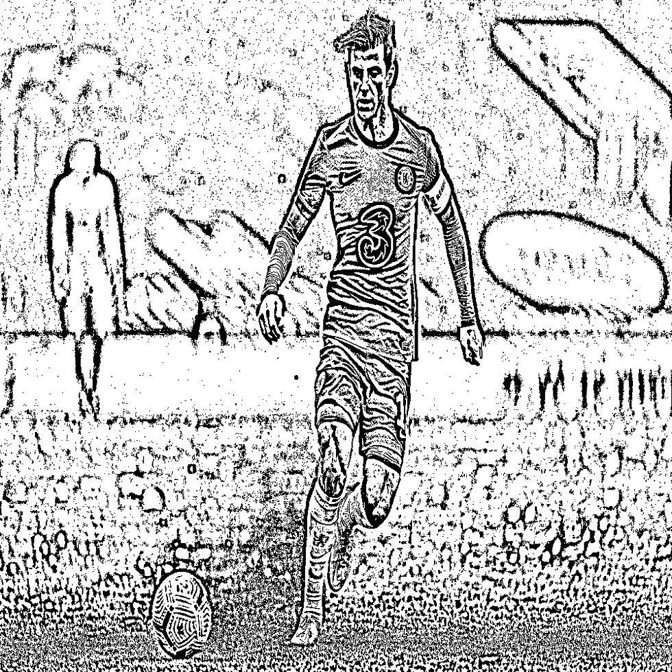
Blurring can be done with cv2.blur() function.
img = cv2.blur (img, (10, 10)) cv2.imshow ('img',img)

For next 2 methods we are going to use image with more noise on it so we can see effects of those methods.
img2 = cv2.imread ('/home/marija/OpenCV/data/noise.png')
cv2.imshow ('img',img2)
There's also a cv2.GaussianBlur() function. Gaussian blurring is highly effective in removing Gaussian noise from an image.
img = cv2.GaussianBlur (img, (5,5), 0) cv2.imshow ('img',img)

Median blur uses cv.medianBlur() function. It takes the median of all the pixels under the kernel area and the central element is replaced with this median value. This is highly effective against salt-and-pepper noise in an image.
img2 = cv2.medianBlur (img2,5) cv2.imshow ('img',img2)
Method cv2.bilateralFilter() is highly effective in noise removal while keeping edges sharp. But the operation is slower compared to other filters. We already saw that a Gaussian filter takes the neighbourhood around the pixel and finds its Gaussian weighted average. This Gaussian filter is a function of space alone, that is, nearby pixels are considered while filtering. It doesn't consider whether pixels have almost the same intensity. It doesn't consider whether a pixel is an edge pixel or not. So it blurs the edges also, which we don't want to do. Bilateral filtering also takes a Gaussian filter in space, but one more Gaussian filter which is a function of pixel difference. The Gaussian function of space makes sure that only nearby pixels are considered for blurring, while the Gaussian function of intensity difference makes sure that only those pixels with similar intensities to the central pixel are considered for blurring. So it preserves the edges since pixels at edges will have large intensity variation.
img2 = cv2.bilateralFilter (img2, 9, 75, 75) cv2.imshow ('img',img2)

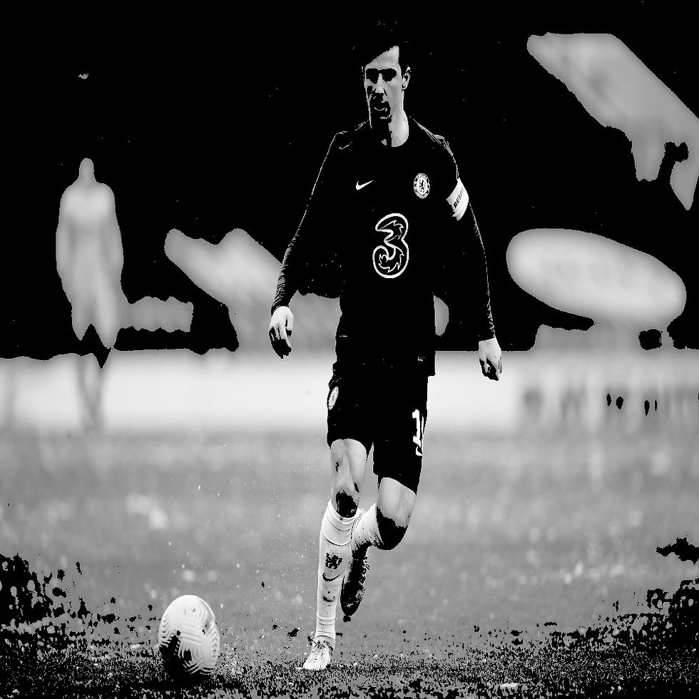
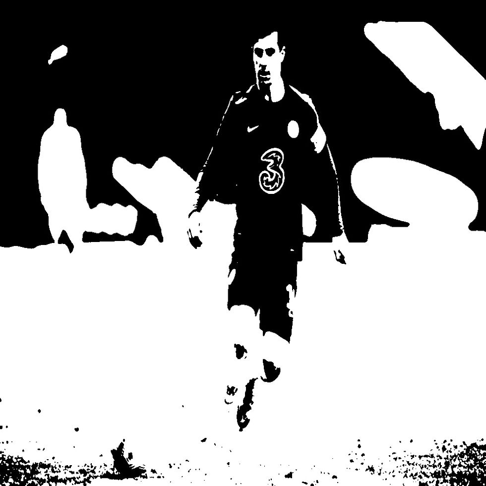
Thresholding can be simple or adaptive. In simple thresholding the same threshold value is applied for every pixel, . If the pixel value is smaller than the threshold, it is set to 0, otherwise it is set to a maximum value. The function cv2.threshold() is used to apply the thresholding. The first argument is the source image, which should always be a grayscale image. The second argument is the threshold value which is used to classify the pixel values. The third argument is the maximum value which is assigned to pixel values exceeding the threshold. The last one is thresholding type and there are: cv2.THRESH_BINARY, cv2.THRESH_BINARY_INV, cv2.THRESH_TRUNC, cv2.THRESH_TOZERO and cv2.THRESH_TOZERO_INV.
First we are going to use cv2.THRESH_BINARY method. So if the pixel value is smaller than the threshold, it is set to 0, otherwise it is set to a maximum value.
img = cv2.cvtColor (img, cv2.COLOR_BGR2GRAY)
_, th1 = cv2.threshold (img, 50, 255, cv2.THRESH_BINARY) cv2.imshow ('th1', th1)

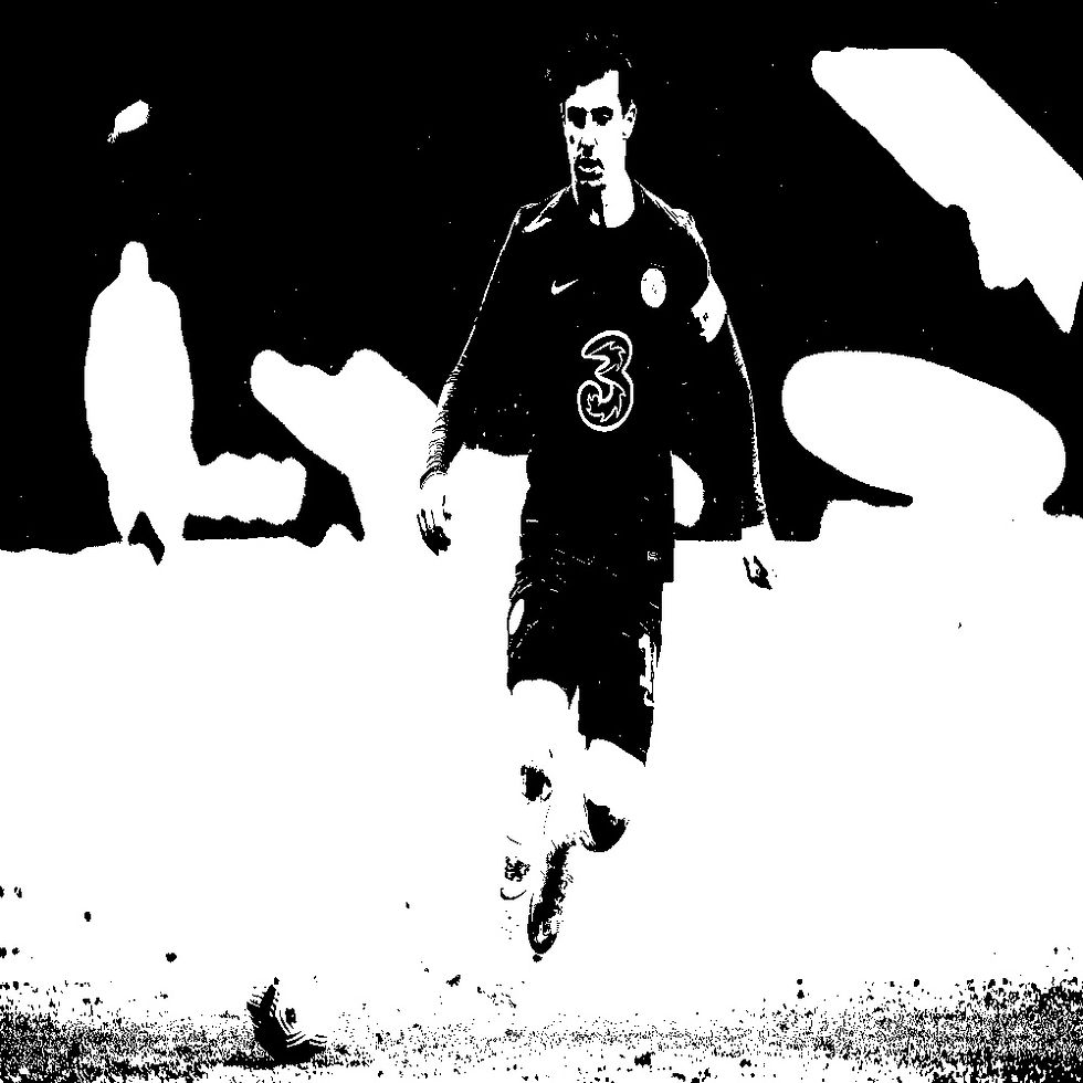
Next, there's cv2.THRESH_BINARY_INV. If the pixel value is smaller than the threshold, it is set to a maximum value, otherwise it is set to 0.
_, th2 = cv2.threshold (img, 200, 255, cv2.THRESH_BINARY_INV) cv2.imshow ('th2',th2)

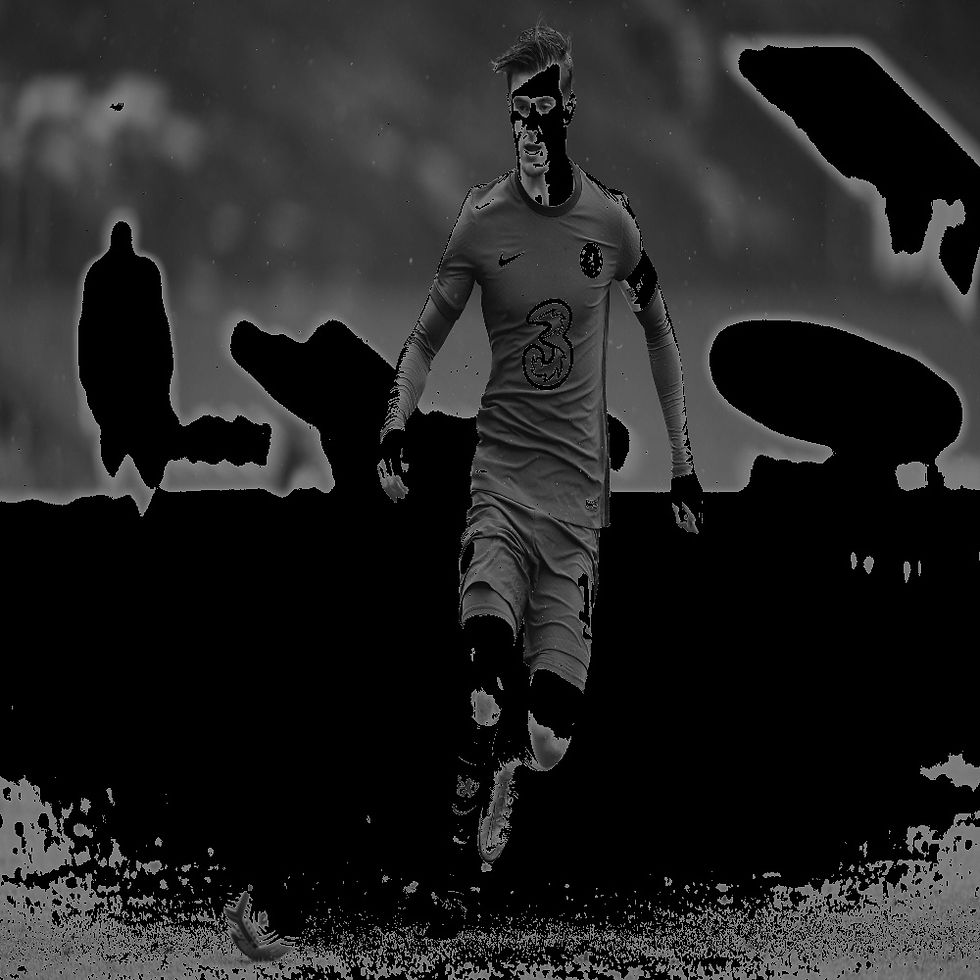
Method cv2.THRESH_TRUNC sets maximum intensity value for the pixels as thresh. If it is greater, then its value is truncated.
_, th3 = cv2.threshold (img, 127, 255, cv2.THRESH_TRUNC) cv2.imshow ('th3',th3)
In method cv2.THRESH_TOZERO, if pixel value is lower than thresh, the new pixel value will be set to 0.
_, th4 = cv2.threshold (img, 127, 255, cv2.THRESH_TOZERO) cv2.imshow ('th4',th4)
The last method cv2.THRESH_TOZERO_INV does the opposite. If pixel value is lower than thresh, the new pixel value will be set to 0.
_, th5 = cv2.threshold (img, 127, 255, cv2.THRESH_TOZERO_INV) cv2.imshow ('th5',th5)
Up until now we used one global value as a threshold. But this might not be good in all cases, e.g. if an image has different lighting conditions in different areas. In that case, adaptive thresholding can help. Here, the algorithm determines the threshold for a pixel based on a small region around it. So we get different thresholds for different regions of the same image which gives better results for images with varying illumination. We will use 6 arguments in function cv2.adaptiveThreshold(). These are image, maxValue, adaptiveMethod, thresholdType, blockSize and C. The blockSize determines the size of the neighbourhood area and C is a constant that is subtracted from the mean or weighted sum of the neighbourhood pixels.
In ADAPTIVE_THRESH_MEAN_C threshold value is the mean of neighborhood area.
th6 = cv2.adaptiveThreshold (img, 255, cv2.ADAPTIVE_THRESH_MEAN_C, cv2.THRESH_BINARY, 11, 2) cv2.imshow ('th6', th6)
In ADAPTIVE_THRESH_GAUSSIAN_C threshold value is the weighted sum of neighborhood values where weights are a Gaussian window.
th7 = cv2.adaptiveThreshold (img, 255, cv2.ADAPTIVE_THRESH_GAUSSIAN_C, cv2.THRESH_BINARY, 11, 2) cv2.imshow ('th7', th7)

In global thresholding, we used an arbitrary chosen value as a threshold. In contrast, Otsu's method avoids having to choose a value and determines it automatically. Otsu's method determines an optimal global threshold value from the image histogram. In order to do so, the cv2.threshold() function is used, where cv2.THRESH_OTSU is passed as an extra flag. The threshold value can be chosen arbitrary. The algorithm then finds the optimal threshold value which is returned as the first output.
_,th8 = cv2.threshold (img, 0, 255, cv2.THRESH_BINARY + cv2.THRESH_OTSU) cv2.imshow ('th8', th8)
Next, we'll use the same function after blurring.
img = cv2.GaussianBlur (img, (5,5), 0) _, th9 = cv2.threshold (img, 0, 255, cv2.THRESH_BINARY + cv2.THRESH_OTSU) cv2.imshow ('th9', th9)
You can check all the code here.


header.all-comments